
Measuring Latent Structural Shear At Model Boundaries Under Non Stationary Sample Noise
Structural shear measures the persistent directional force warping model parameters along domain boundaries when non stationary noise obscures local loss gradients.

Seam
An optimization model deployed into dynamic input environments encounters structural tension where defined system rules meet raw input data. In non-stationary processing, input distributions shift continually across time windows, producing localized fluctuations in residual errors. System operators frequently treat these localized spikes as transient background disturbance.
The underlying transfer function, however, experiences localized mechanical strain when sample noise overlays true operational boundary shifts.

Latent Force Allocation across Domain Edges
Mechanical stress accumulates along internal lines long before material failure occurs. Structural shear represents the directional differential between predicted loss gradients and actual physical path resistance. Value sets the baseline axis.
When an operational model evaluates incoming data, optimization algorithms follow the descent trajectory offering minimal short-term computational cost. Noise hides stress. In non-stationary environments, dynamic noise profiles generate variable variance envelopes that mask underlying parameter misalignments.
The system routes around high-resistance computations, concentrating unprocessed structural strain along outer domain perimeters.
Consider an operational model built for real-time asset pricing under shifting market liquidity. The model assumes stationary variance across execution intervals. Over a six-month period, liquidity volatility doubles while mean values remain constant.
Standard validation metrics register minor loss increases, treating the variance as random sample noise. Beneath the surface, the boundary parameter weights warp to accommodate short-term noise spikes, creating severe latent shear along margin limits. The system maintains surface stability while internal mechanical capacity degrades.
Non stationary variance obscures localized gradient shifts whenever the sampling window undercounts boundary crossings.

Boundary Deformation under Variable Sample Distribution
Mathematical models construct implicit perimeters around high-density sampling zones. When sample noise becomes non-stationary, the effective boundary expands and contracts irregularly across successive processing intervals. Boundaries carry weight.
Parameter weight vectors optimized for central sample densities struggle to maintain accuracy along these oscillating edges. The model experiences localized shear as gradient updates in low-density zones collide with frozen weights established during high-density historical windows.
Systematic measurement of boundary deformation isolates sample noise from true structural shear. The operator evaluates the directional derivative of the loss surface relative to parameter boundaries across discrete temporal windows. When the directional derivative exhibits persistent alignment bias despite zero-mean noise distributions, structural shear is present.
Ignoring this directional bias allows latent shear to build until the model encounters unmodeled input territory.
When the dynamic window threshold is set to zero, the shear calculation converts structural deformation directly into baseline drift.

Gauge
Quantitative evaluation of structural strain demands continuous tracking of differential residual vectors across shifting inputs. Traditional metrics rely heavily on global error metrics such as mean squared error or aggregate log-loss. Global loss metrics blend internal structural misalignment with background noise, concealing localized boundary failure.
Shear builds quietly. A targeted evaluation metric separates stationary input variance from structural directional displacement along model boundaries.
Evaluating Gradient Variance along Boundary Extremes
Gradient vectors calculated near operational limits reveal the internal forces acting upon model weights. The gradient of a loss function indicates the path of steepest ascent, marking the exact direction of maximum computational friction. In non-stationary noise environments, local gradient directions oscillate rapidly.
Calculating a temporal moving average of unit gradient vectors isolates the persistent structural directional force from transient stochastic movement. The magnitude of this averaged vector measures latent structural shear.
High structural shear values indicate that the optimization trajectory is repeatedly deflected by rigid boundary parameters. The system avoids computing solutions in high-shear regions, accumulating unprocessed material behind its built limits. Shear diagnostic procedures require tracking several distinct boundary failure modes across operation cycles.
- Distributional Splice Deficit occurs when continuous updates truncate boundary residuals before structural convergence settles.
- Variance Smoothing Failure arises when high-pass filtering suppresses structural shear signals alongside background sample noise.
- Asymmetric Boundary Creep happens when optimization steps favor low-cost regions, leaving dense unprocessed error vectors along outer limits.
Local shear vectors reveal boundary stability far faster than global loss averages.
Measurement Vectors for Non Stationary Streams
Analyzing non-stationary streams involves establishing sliding observation windows calibrated to the expected drift rate of the sample noise. Standard sliding windows fail when noise variance shifts faster than the window duration. Vectors map the slope.
An adaptive measurement window adjusts its duration based on the second moment of the input residual distribution. Short windows isolate rapid noise bursts, while extended windows expose slow, systemic shear accumulation along domain boundaries.
Data moves constantly. Evaluating model structural health involves mapping local shear values against the baseline axis. When local shear magnitude exceeds threshold constraints, the system experiences structural deformation, altering how the model processes edge-case inputs.
Misinterpreting structural shear as sample noise leads directly to uncalibrated predictions that fail catastrophically upon encountering novel distribution bounds.

Drift
Non-stationary environments generate time-varying noise distributions that obscure structural changes within the underlying data generator. System operators routinely misclassify structural changes as continuous baseline drift, applying global model recalibrations that fail to address boundary-specific deformation. Baseline recalibration shifts the entire loss surface, altering parameter weights in stable regions while leaving high-shear boundary zones fundamentally uncorrected.
Is Non Stationary Noise Masking Surface Stress?
Decoupling environmental noise shifts from structural model deformation requires analyzing residual distributions across orthogonal spatial vectors. Noise hides stress. When input sample noise changes its primary covariance structure, the error surface deforms unevenly.
The model adjusts its weights along the path of least resistance, shifting structural strain onto perimeter nodes. This redistribution creates localized zones of extreme tension where model assumptions conflict with non-stationary realities.
Tracking the evolution of boundary residuals over sequential processing steps reveals whether error increases stem from input noise variance or structural shear. The baseline shifts. If residual error vectors maintain a consistent spatial orientation while noise variance scales, structural shear is the primary driver of model degradation.
An expanding error envelope along model limits signals hidden structural shear before performance metrics degrade.
Temporal Decay of Boundary Confidence
Model confidence estimates degrade rapidly when structural shear remains uncorrected under non-stationary noise. Boundary parameters established on historical input distributions lose statistical validity as sample noise alters local curvature. The baseline stays fixed while input realities shift underneath.
The operator maps temporal boundary decay through a structured evaluation sequence.
- Establish a moving baseline for input noise across centered time blocks.
- Isolate localized boundary residuals from global system variance.
- Project residual vectors against known physical constraint surfaces.
Errors accumulate here. The sequence reveals the precise spatial regions where model boundaries no longer hold structural integrity. The operator measures the unspent volume of uncomputed residual force to determine reinforcement parameters.
The precise point where non-stationary sample noise completely swallows the signal of boundary degradation remains unidentified for non-linear loss surfaces.
Plate
Diagnostic tools for structural assessment vary significantly in their mathematical foundations, computational overhead, and sensitivity to non-stationary sample noise. Selecting an appropriate diagnostic method requires balancing the computational cost of continuous gradient evaluation against the risks of undetected boundary shear failure. The wall stays rigid.
Comparing diagnostic performance across controlled stress regimes establishes clear criteria for deployment.

Comparative Mechanics of Shear Diagnostic Instruments
Diagnostic tools monitor structural stress by evaluating model performance across distinct analytical dimensions. Windowed residual projection monitors local variance shifts over bounded temporal windows. Boundary kernel density estimation evaluates sample distribution density along model limits.
Non-parametric gradient shear mapping measures directional gradient divergence across shifting noise environments.
| Diagnostic Method | Primary Input Vector | Noise Tolerance Threshold | Computation Cost | Primary Shear Marker |
|---|---|---|---|---|
| Windowed Residual Projection | Scalar Loss History | Low Sample Variance | Low Computational Overhead | Variance Spike Duration |
| Boundary Kernel Density Estimation | Spatial Sample Coordinates | Moderate Distribution Shift | Medium Computational Overhead | Local Density Deficit |
| Non-Parametric Gradient Shear Mapping | Directional Gradient Tensor | High Non-Stationary Noise | High Computational Overhead | Vector Alignment Bias |
Selecting a diagnostic strategy depends on the underlying noise profile of the operational environment. High-frequency non-stationary noise environments demand non-parametric gradient shear mapping to isolate structural displacement from temporary stochastic variance. Environments with predictable noise bounds achieve sufficient shear detection using windowed residual projections at significantly lower computational expense.
Structural Alignment versus Surface Variance
Surface variance reflects temporary fluctuations in input data quality, whereas structural alignment reflects the internal coherence between model parameter assumptions and physical environment rules. Cost rises fast. Optimization algorithms exposed to high surface variance frequently over-correct parameter weights, introducing severe structural shear along domain limits.
The system achieves short-term loss reductions by warping its internal geometry, creating brittle boundaries susceptible to sudden failure.
Measuring latent potential involves calculating the inverse gradient vector along high-shear boundaries. This inverse vector represents the unspent structural capacity of the system, identifying zones where model updates yield maximum stability gains. The seam splits.
Reinforcing model boundaries along latent potential vectors restores structural balance under persistent non-stationary sample noise.
Boundary models degrade along the exact path the optimization system routinely routes around.
High model accuracy metrics across training slices often cover deep structural weaknesses along the deployment boundary.

Rupture
Structural shear accumulation eventually leads to boundary rupture when local stress exceeds parameter weight tolerance limits. Rupture manifests as sudden, non-linear degradation of predictive capability when input data crosses high-shear domain perimeters. The system encounters unmodeled territory, failing to generate valid outputs because its internal parameter geometry cannot accommodate the input vector configuration.

System Failure Mechanics at Boundary Limits
Rupture events occur without explicit warning when monitoring frameworks evaluate global metrics exclusively. Global metrics remain stable while boundary shear consumes internal reserve capacity. When input distributions shift into high-shear zones under non-stationary noise, the model experiences instantaneous accuracy collapse.
The model holds until the edge snaps.
Preventing catastrophic boundary rupture requires setting structural reinforcement parameters derived from latent potential measurements. The operator enforces structural boundaries through targeted optimization constraints, forcing parameter updates to absorb structural shear rather than transferring strain to perimeter nodes.
Reclaiming Latent Potential Behind Built Boundaries
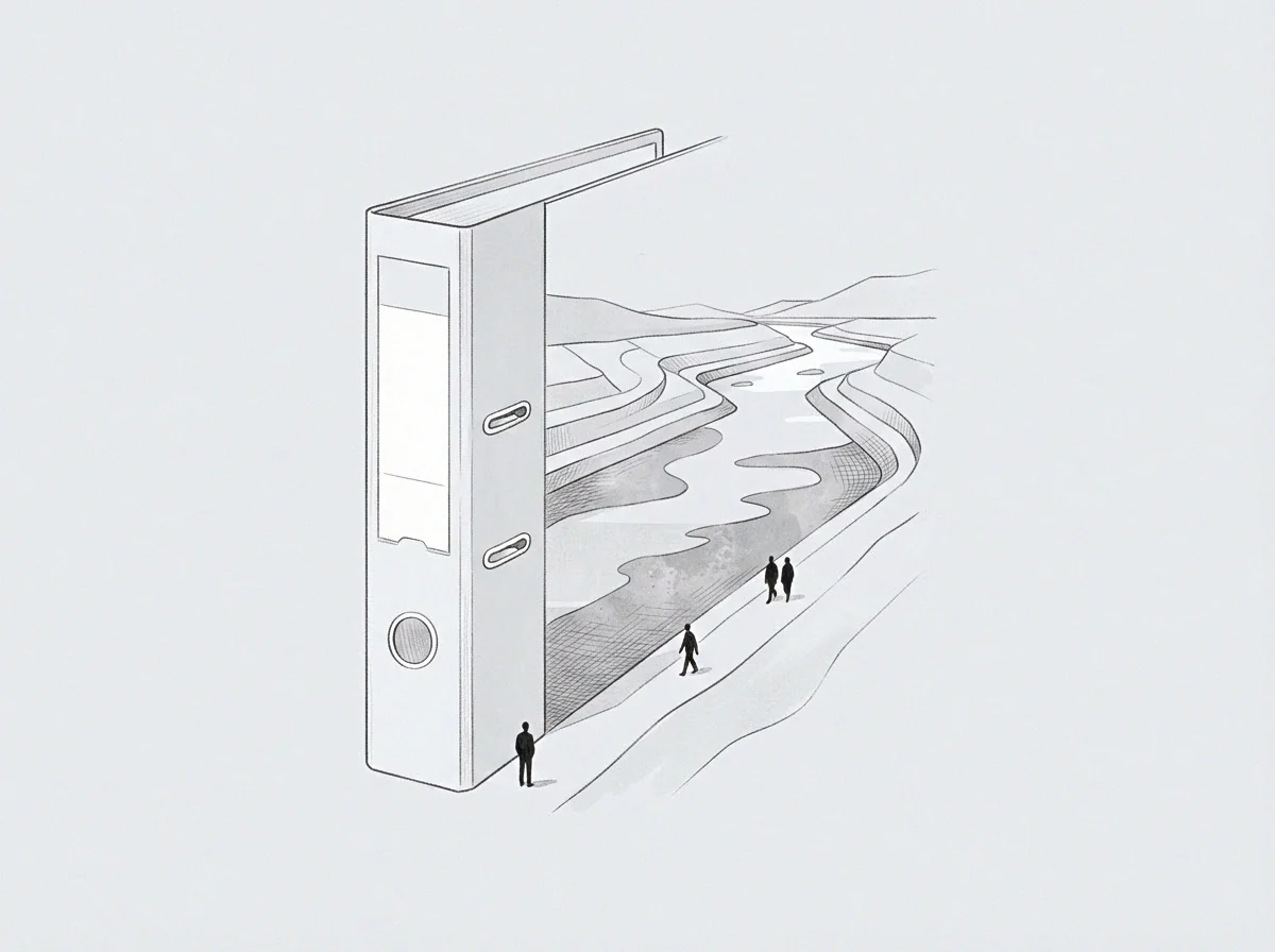
Behind built model boundaries lies an unspent volume of uncomputed structural capacity. Avoiding computations in high-resistance domain regions creates dark zones within the model’s operational space. Reclaiming this latent potential requires reversing the optimization descent vector along high-shear boundaries, forcing the system to process accumulated residual material.
- Boundary Isolation limits error propagation by decoupling localized non-stationary noise from core gradient updates.
- Latent Path Projection maps unspent boundary potential directly into the ascent gradient vector.
- Residual Recalibration restores predictive accuracy by adjusting parameter weights against physical limits rather than noisy sample averages.
System operators who monitor boundary shear continuously adjust gradient steps before material failure occurs. The unspent latent volume behind the boundary becomes the explicit input for the next optimization pass.