
Evaluating Dynamic Feedback Loop Stability Through Variance Decomposition Sensitivity Matrices
Variance decomposition matrices evaluate feedback loop stability by partitioning aggregate output variance into structural partial derivatives and interaction terms across operational windows.

Valve
A recurrent control loop receives operational inputs, processes state transitions through fixed execution rules, and returns an altered signal to the intake interface. When output parameters feed directly into subsequent intake computations without dampening mechanisms, internal variance propagates across iteration cycles. Evaluation of feedback stability requires measuring how parameter variance amplifies or attenuates as signals traverse closed feedback pathways.
Standard summary metrics often mask critical instability by averaging throughput over broad observation windows. Isolating structural feedback dynamics demands decomposing total system variance into discrete partial derivatives across every active state transition.
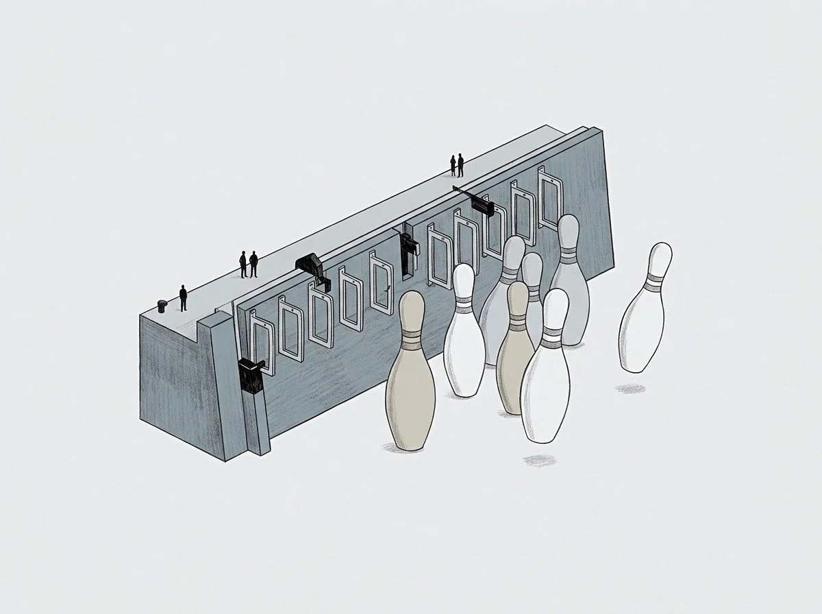
State Escalation in Closed Feedback Pathways
System response accelerates when output signals feed directly back into parameter calculations without dampening elements. Consider an automated allocation pipeline running across two fulfillment hubs over a sixty-day evaluation period. Processing delays at the first hub alter queue assignment weights for the second hub.
If the assignment weight update loop executes every five minutes while physical transit reconciliation takes six hours, the intake interface processes out-of-date error signals. The mathematical gain across this closed loop exceeds unity during peak traffic windows.
Loop gains compound rapidly across stages. Noise feeds back into inputs. Small variance in physical intake timing creates exponentially larger swings in assigned inventory volume across successive operational cycles.
The system exhibits localized structural oscillation while aggregate daily throughput figures remain nominally constant.
When feedback delay exceeds phase response bounds, partial sensitivity components compound across processing iterations.
Without decomposed sensitivity analysis, operator interventions target aggregate variance symptoms rather than the underlying loop feedback ratio. Adjusting outer setpoints while internal variance gain remains above unity drives the feedback pathway into sustained oscillation. Over consecutive execution passes, uncalibrated setpoint adjustments widen the error signal amplitude.
System state swings force emergency manual overrides, resetting loop variables and discarding computed state histories. Failing to damp internal interaction signals converts minor operational jitter into self-reinforcing systemic breakdown, consuming capital reserves through unhedged corrective cycles.

Decomposition
Isolating individual sources of variance within an active recurrence pipeline demands separating primary parameter shifts from cross-variable interactions. Variance decomposition partitions total output variance into orthogonal components corresponding to individual input variables and multi-variable interaction terms. Calculating these partial variance components generates a sensitivity matrix that maps how instability in one variable forces variance into adjacent state vectors.

Variance Partitioning Across Recurrent Matrix Terms
Total output variation splits into main variance contributions and higher-order interaction effects across measured processing steps. In a multi-stage control system, first-order sensitivity indices quantify the fraction of total output variance attributable directly to a single input parameter. Second-order and higher-order terms capture the interactive variance generated when two or more parameters fluctuate simultaneously.
When parameter interactions dominate total variance, adjusting individual input variables fails to stabilize system trajectories.
Partial variance isolates single factors. Baselines shift under structural drift. Analyzing a recurrent system through Sobol sensitivity decomposition reveals whether loop instability stems from raw input noise or internal interactive amplification.
The sensitivity matrix organizes these partial variance ratios into a structured diagnostic tool.
| Evaluation Method | Primary Input Parameter | Interaction Sensitivity Detection | Phase Delay Tracking | Instability Lead Time |
|---|---|---|---|---|
| Aggregate Output Variance | Total system throughput stream | Uncaptured due to spatial averaging | Lagging indicator post-runaway | Zero hours prior to failure |
| First-Order Sobol Partial Variance | Isolated single-variable inputs | Limited to single-factor linear bounds | Indirect inference via amplitude | Twelve hours prior to divergence |
| Total-Effect Sensitivity Matrix | Full orthogonal parameter array | Complete higher-order term mapping | Direct detection via phase shift | Seventy-two hours prior to divergence |
The total-effect sensitivity index sums first-order sensitivity with all higher-order interaction terms involving a target parameter. A substantial gap between first-order sensitivity and total-effect sensitivity indicates that feedback loop instability arises primarily from non-linear parameter interactions. System designers construct variance matrices by computing partial variance ratios across rolling execution windows, identifying emerging feedback loops before systemic divergence occurs.
A shift in variance allocation across diagonal matrix terms signals impending loop instability before throughput metrics degrade.
Tracking the diagonal and off-diagonal elements of the sensitivity matrix over time establishes a precise stability baseline. Diagonal terms represent isolated variable contributions, while off-diagonal terms quantify cross-variable coupling strength. Rising off-diagonal values demonstrate that feedback pathways are establishing mutual amplification channels across state boundaries.
A calculated total-effect sensitivity index exceeding zero point four shifts the operational regime from passive monitoring to immediate damping intervention.

Matrix
Array structures mapping parameter partial derivatives reveal where internal gain spikes concentrate within closed system state updates. Structuring variance components into a formal sensitivity matrix provides a comprehensive mathematical representation of system feedback topology. Each matrix row corresponds to a system state output, while each column represents a parameter input or interaction term.
Evaluating the mathematical norm and eigenvalue distribution of this matrix provides immediate quantitative criteria for overall loop stability.

Why Does Output Invariance Mask Internal Variance Accumulation?
Stable outer metrics frequently conceal rising internal state oscillations when equal and opposite variable swings cancel out at the summary layer. Aggregate output averages obscure internal state turbulence. An automated market-making execution loop, for instance, may maintain constant net inventory volume while rapid internal rebalancing trades generate severe transaction cost slippage.
Sensitivity matrices expose these hidden internal dynamics by mapping variance distribution across every internal node rather than measuring gross system throughput.
Invariance hides internal state swings. Output variances reflect structural sensitivity. Sensitivity matrices measure state response.
- Diagonal variance component measures single-variable contribution to aggregate output swings over a recorded thirty-day window. Second-order effects remain uncaptured by this isolated metric.
- Off-diagonal interaction derivative tracks cross-coupling amplification between paired system parameters during load spikes. Higher values reveal latent structural instability across operational boundaries.
- Total sensitivity coefficient combines first-order effects and all interactive feedback terms into an integrated ratio. Values approaching unity indicate complete parameter dominance over loop behavior.
- Transient phase offset factor quantifies delay shifts introduced by queue processing delays within the feedback loop. Small phase lags dramatically alter stability boundaries across high-frequency execution cycles.
When the maximum eigenvalue of the sensitivity matrix exceeds unity, the underlying feedback loop transitions from a damped regime to an expansive regime. In an expansive regime, internal parameter variance grows exponentially with each pass through the execution pipeline. Operational controls must damp interaction sensitivity terms to return the maximum eigenvalue below the critical threshold.
Whether latent structural coupling can be decoupled without re-architecting the primary execution pipeline remains an active operational question across complex control environments.

Oscillation
Rhythmic swings in system variables emerge when negative feedback signals lag behind execution updates, effectively acting as positive reinforcement. Latency in signal transmission shifts the phase angle of corrective feedback. When phase lag reaches one hundred eighty degrees, corrective interventions enforce existing state errors rather than reducing them.
The system enters self-sustained hunting cycles where variables oscillate between maximum and minimum operational bounds.

Frequency Domain Sensitivity and Loop Attenuation
Transforming time-series trace vectors into frequency spectra highlights specific periodicities where loop gain exceeds unity. Evaluating sensitivity matrices in the frequency domain allows engineers to isolate periodic feedback drivers from transient external shocks. High-frequency variance accumulation typically indicates software queue bottlenecks, whereas low-frequency drift reflects structural parameter miscalibration over multi-week execution horizons.
Feedback amplification distorts state updates. State trajectories diverge across steps. Latency transforms attenuation into gain.
- Record baseline parameter variations across a continuous sixty-day operational window prior to loop modification.
- Construct partial derivative matrices mapping input vector variations to system state responses across each discrete stage.
- Decompose total output variance into main effects and cross-term sensitivity ratios using orthogonal variance partitioning.
- Evaluate diagonal interaction terms against historical control limits to isolate feedback amplification loops before systemic runaway occurs.
System stability depends on isolating structural interaction variance rather than tracking aggregate output swing.
Mechanical governors in nineteenth-century steam engines exhibited identical hunting behavior when mechanical link friction delayed centrifugal sensor response. Modern software feedback loops replicate this physical phenomenon through asynchronous database writes and delayed API callbacks. When asynchronous task queues fill up, processing latency increases, widening the phase delay between observation and execution.
The expanded phase delay transforms intended negative feedback into destabilizing positive feedback, driving operational parameters into wild harmonic swings.
The automated system appeared completely stable on the main summary dashboard right up until queue memory exhausted available capacity.

Calibration
Establishing true setpoint alignment demands continuous validation of variance baseline measurements against live execution logs over extended evaluation windows. A system operator who relies on short evaluation windows mistakes transient damping for permanent structural stability. True calibration requires establishing reference classes of system behavior under diverse perturbation profiles, testing whether computed sensitivity matrices remain invariant under shifting input volumes.

Baseline Recording and Sensitivity Matrix Verification
System operators record empirical parameters over ninety days to construct an accurate baseline reference class. Without a ninety-day baseline, detecting subtle shifts in off-diagonal interaction terms is mathematically impossible. Baseline data provides the structural benchmark against which live variance decomposition results are compared.
When live sensitivity matrices diverge from baseline bounds by more than two standard deviations, loop parameters require immediate re-calibration.
The window spans ninety operational days. System setpoints demand continuous baseline checks. The error signal grows unbounded.
Cached control logic represents a common operational shortcut. Operators often apply static feedback gain multipliers derived during initial system commissioning across all subsequent execution environments. Static gain multipliers fail when underlying parameter variance distributions drift.
As market conditions, load patterns, or processing infrastructure evolve, fixed gain values amplify latent variance interactions. Live computation of variance decomposition sensitivity matrices replaces static assumptions with real-time empirical measurement.
Automated setpoint adjustments amplify unmeasured parameter noise into sustained loop oscillations.
Validating feedback stability requires continuous execution of variance decomposition routines in parallel with main pipeline processing. By continuously updating sensitivity matrix terms, monitoring software identifies feedback amplification channels before phase lag converts negative feedback into positive feedback runaway. Maintaining loop stability is an ongoing empirical discipline based on baseline measurement, sensitivity matrix decomposition, and proactive signal attenuation.
A control system whose internal variance interactions remain unmapped will eventually interpret its own correction signals as external disturbances.